
Numbers alone can be difficult to interpret. Conditional Formatting turns data into visual insights instantly.
What is Conditional Formatting?
It highlights cells based on conditions.
What it is used for
- Identifying trends
- Highlighting top values
- Detecting errors
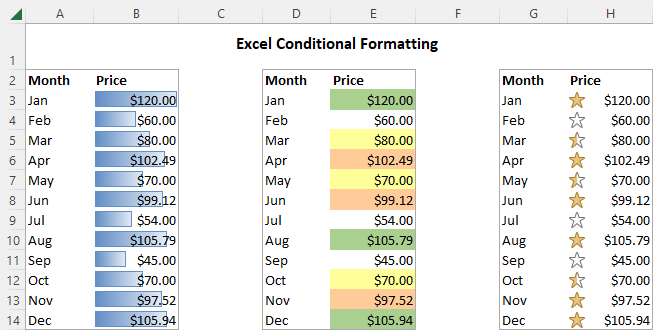
Types of Formatting
- Color scales
- Data bars
- Icon sets
How to use conditional formatting in Excel
To truly leverage the capabilities of conditional format, you need to learn how to utilize various rule types. The good news is that whatever rule you are going to apply, it defines the two key things:
- What cells are covered by the rule.
- What condition should be met.
So, here’s how you use Excel conditional formatting:
- In your spreadsheet, select the cells you want to format.
- On the Home tab, in the Styles group, click Conditional Formatting.
- From a set of inbuilt rules, choose the one that suits your purpose.
As an example, we are going to highlight values less than 0, so we click Highlight Cells Rules > Less Than…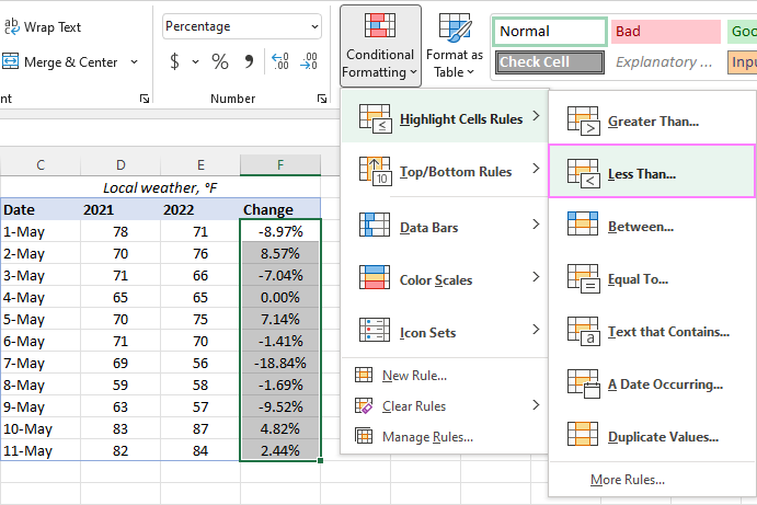
- In the dialog window that appears, enter the value in the box on the left and choose the desired format from the drop-down list on the right (default is Light Red Fill with Dark Red Text).
When done, Excel will show you a preview of formatted data. If you are happy with the preview, click OK.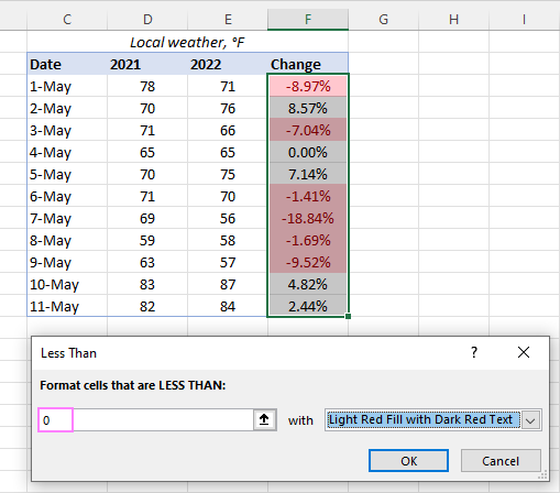
In a similar manner, you can use any other rule type that is more appropriate for your data, such as:
- Greater than or equal to
- Between two values
- Text that contains specific words or characters
- Date occurring in a certain range
- Duplicate values
- Top/bottom N numbers
Using Formula-Based Rules
Example:
=A1>100
Used for advanced highlighting.
Conclusion
Conditional Formatting helps users understand data quickly without complex analysis.