
When working with large datasets in Microsoft Excel, finding specific information quickly can become difficult. This is where Filtering becomes extremely useful. Filtering allows users to display only the data that meets specific criteria while hiding the rest.
Instead of manually searching through hundreds or thousands of rows, Excel’s filtering feature enables you to analyze your data efficiently and make faster decisions.
What is Filtering in Excel?
Filtering is a feature that allows users to show only the rows that match certain conditions while temporarily hiding the other rows.
For example, you can filter data to show:
- Sales from a specific region
- Products above a certain price
- Employees from a particular department
- Records from a specific date range
Filtering does not delete data. It simply hides rows that do not meet the selected conditions.
How to Apply Filters in Excel
Applying a filter in Excel is very simple.
Follow these steps:
- Select the dataset including the column headers.
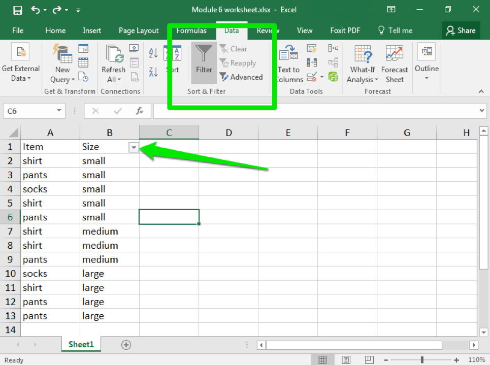
- Go to the Data tab on the Excel ribbon.
- Click Filter.
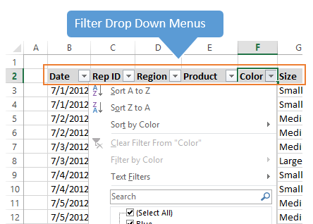
- Small dropdown arrows will appear in each column header.
You can now filter your data based on values in each column.
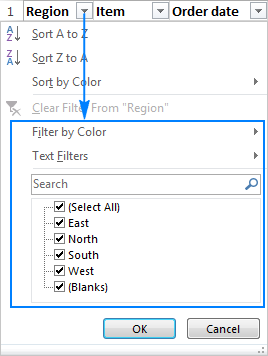
Filtering by Specific Values
One of the most common ways to filter data is by selecting specific values.
For example, if you have a sales dataset with regions such as:
- North
- South
- East
- West
You can filter the column to show only North region sales.
Steps:
- Click the filter arrow in the column header.
- Uncheck Select All.
- Select the value you want.
- Click OK.
Excel will now display only rows containing that value.
Using Number Filters
Excel also allows filtering based on numeric conditions.
Examples include:
- Greater than
- Less than
- Between values
- Top 10 items
Example scenario:
Filter a sales dataset to display sales greater than $5,000.
Steps:
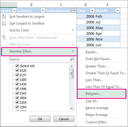
- Click the filter dropdown in the column.
- Select Number Filters.
- Choose Greater Than.
- Enter the value (5000).
Using Text Filters
Text filters are useful when working with names, categories, or descriptions.
Excel provides options such as:
- Contains
- Does not contain
- Begins with
- Ends with
Example:
Filter a customer list to show names that start with the letter A.
Steps:
- Click the filter dropdown.
- Select Text Filters.
- Choose Begins With.
- Enter the letter A.
Excel will display only matching results.
Filtering by Color
Excel allows users to filter rows based on cell color or font color.
This is useful when conditional formatting is applied.
Example:
If high-performing sales are highlighted in green, you can filter to show only those rows.
Steps:
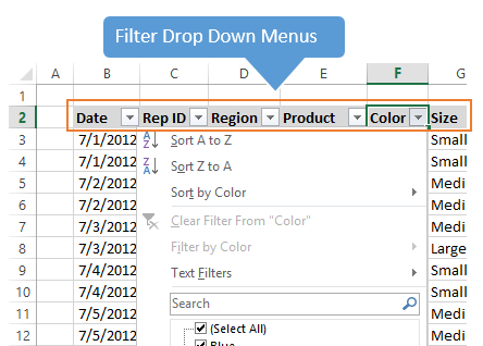
- Click the filter arrow.
- Select Filter by Color.
- Choose the desired color.
Clearing Filters
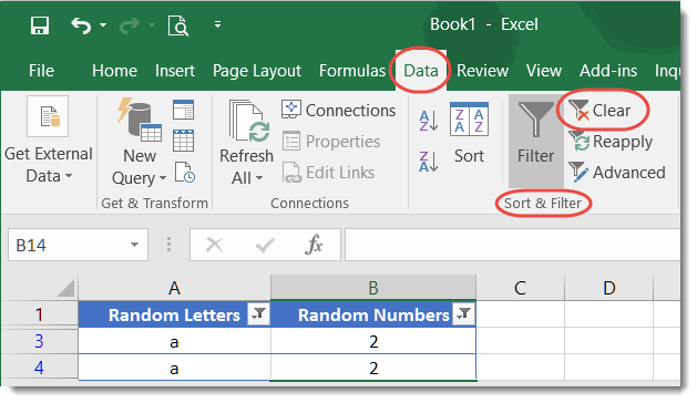
To remove filters and display all data again:
- Go to the Data tab.
- Click Clear.
This restores the dataset to its original state.
Benefits of Using Filters
Filtering provides several advantages when working with Excel datasets.
These include:
- Faster data analysis
- Easier navigation through large datasets
- Ability to focus on specific information
- Improved decision-making
Filtering is particularly useful for:
- Sales reports
- Financial analysis
- Customer databases
- Inventory tracking
Common Mistakes When Using Filters
While filtering is simple to use, some common mistakes include:
- Not selecting the full dataset before applying filters
- Forgetting that filters are active
- Filtering columns with inconsistent data
Always ensure your dataset has clear column headers and consistent formatting before applying filters.
Conclusion
Filtering is one of the most powerful and commonly used features in Microsoft Excel. It allows users to quickly isolate relevant information from large datasets without altering the original data.
By mastering Excel’s filtering tools, you can analyze information faster, uncover insights more easily, and work more efficiently with your data.