
Data is powerful, but only when it is presented clearly. Raw tables and numbers can be difficult to interpret, especially for decision-makers. This is where interactive dashboards come in.
An Excel dashboard transforms complex data into visual, interactive, and easy-to-understand insights. The best part? You don’t need coding skills to build one.
In this article, you’ll learn how to create a fully interactive dashboard in Excel using built-in tools like charts, Pivot Tables, and slicers.
What is an Excel Dashboard?
An Excel dashboard is a visual representation of key data and metrics in one place. It typically includes:
- Charts
- Tables
- KPIs (Key Performance Indicators)
- Filters or slicers
Dashboards help users quickly monitor performance and make data-driven decisions.

Why Use Dashboards in Excel?
Dashboards are widely used in business because they:
- Simplify complex data
- Highlight important trends
- Improve decision-making
- Save time on reporting
- Provide real-time insights
Instead of scrolling through multiple sheets, everything is displayed in one place.
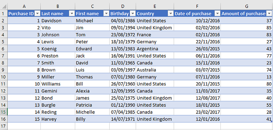
Step 1: Prepare Your Data
Before creating a dashboard, your data must be clean and organized.
Ensure that:
- There are no blank rows or columns
- Each column has a clear header
- Data is structured in a table format
Well-structured data is the foundation of a good dashboard.
Step 2: Create Pivot Tables
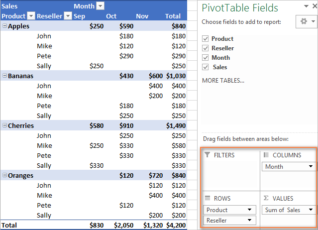
Pivot Tables are used to summarize and analyze data.
Steps:
- Select your dataset
- Go to the Insert tab
- Click PivotTable
- Choose where to place it
Use Pivot Tables to calculate:
- Total sales
- Average values
- Counts
- Grouped data
Step 3: Add Charts
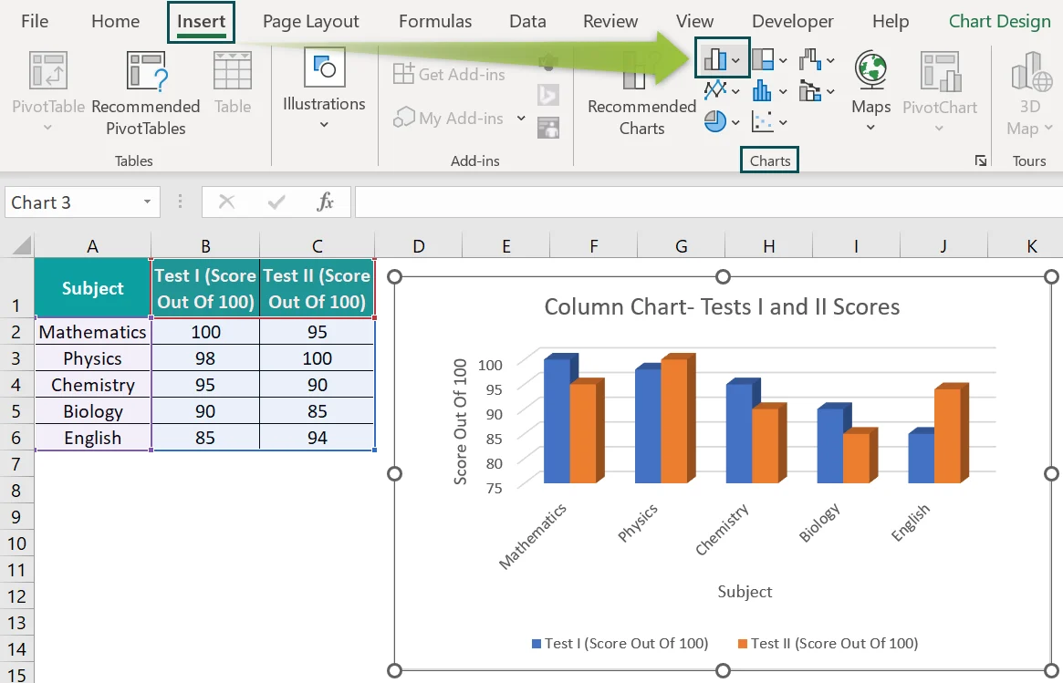
Charts turn your summarized data into visuals.
Common dashboard charts include:
- Bar charts
- Line charts
- Pie charts
- Column charts
Steps to create a chart:
- Select your Pivot Table
- Go to the Insert tab
- Choose a chart type
Charts help users quickly understand trends and patterns.
Step 4: Add Slicers for Interactivity
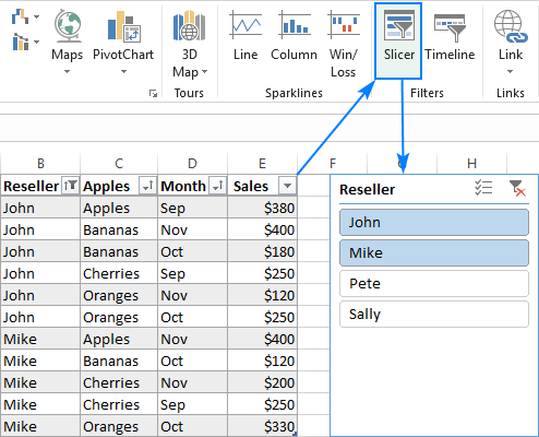
Slicers allow users to filter data interactively.
Steps:
- Click your Pivot Table
- Go to the Insert tab
- Click Slicer
- Select fields (e.g., Region, Product)
Slicers create clickable buttons that filter your dashboard instantly.
Step 5: Create KPI Cards
KPI cards display key metrics such as:
- Total Sales
- Profit
- Number of Customers
You can create KPIs using simple formulas like:
=SUM(B2:B100)
Format the result using large fonts and bold styles to make it stand out.
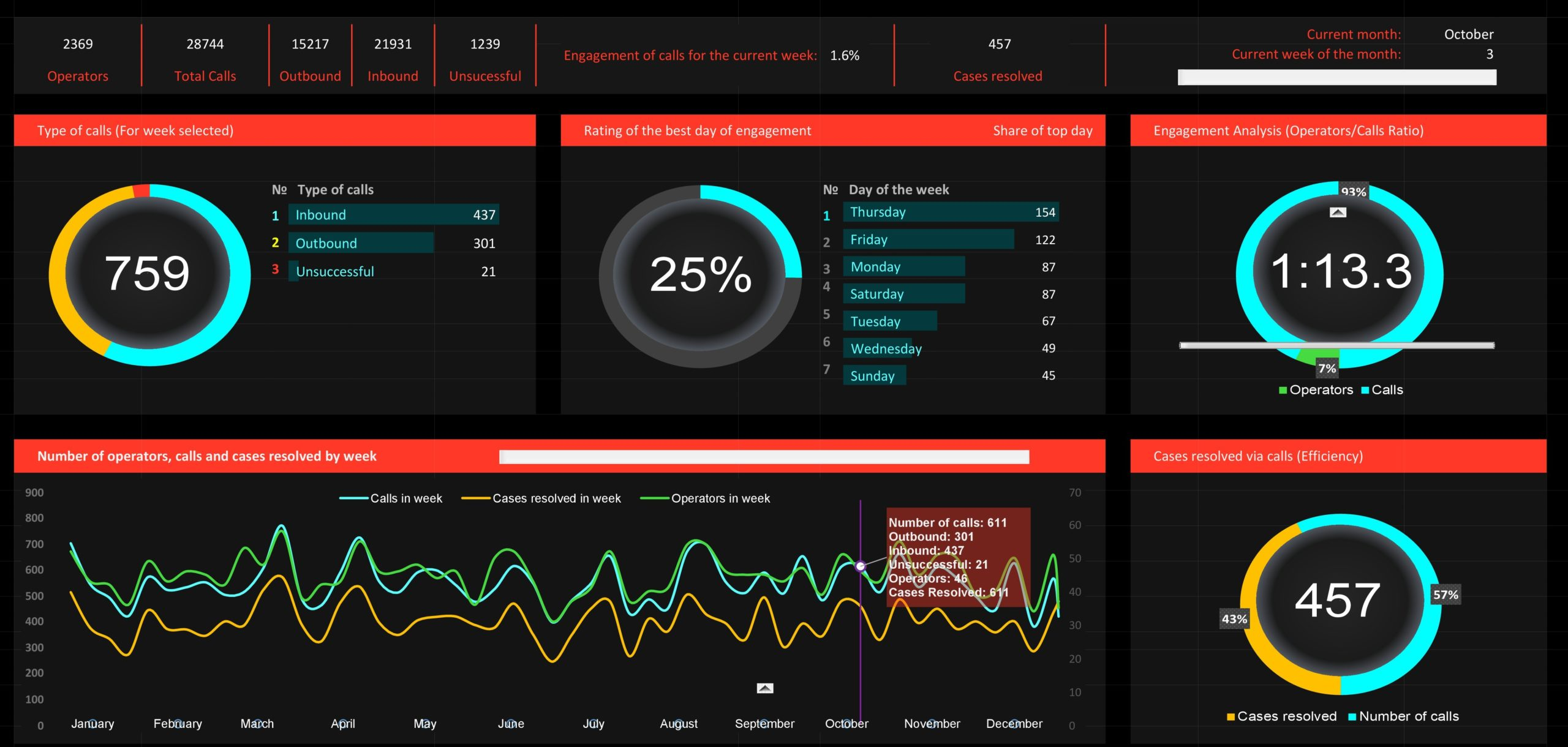
Step 6: Design Your Dashboard Layout
A good dashboard is not just functional — it is visually appealing.
Tips for layout:
- Place KPIs at the top
- Group related charts together
- Use consistent colors
- Leave enough spacing
Keep the design clean and uncluttered.
Step 7: Make It Dynamic
To make your dashboard fully interactive:
- Connect slicers to multiple Pivot Tables
- Use dynamic charts
- Update data regularly
- Use Excel Tables for automatic expansion
This ensures your dashboard updates automatically when data changes.
Best Practices for Excel Dashboards
To build effective dashboards:
- Focus on key metrics only
- Avoid overcrowding visuals
- Use simple chart types
- Maintain consistency in colors and fonts
- Test interactivity
A simple dashboard is often more effective than a complex one.
Common Mistakes to Avoid
- Using too many charts
- Including unnecessary data
- Poor alignment and spacing
- Lack of clear labels
Always design dashboards with the end user in mind.
Conclusion
Building interactive dashboards in Excel allows you to transform raw data into meaningful insights. By combining Pivot Tables, charts, slicers, and good design principles, you can create professional dashboards without writing any code.
Mastering this skill will not only improve your data analysis capabilities but also make your reports more impactful and easier to understand.