
We all love beautiful things don’t we? Formatting in Excel helps us achieve exactly that. We can make our spreadsheets more presentable. We will use the data in the arithmetic operations table. We will make the column names;
- Bold
- Align serial numbers to the left
-
Enclose the data in boxes.
Make column names bold
- Highlight the cells that have the column names by dragging them.
- Click on the bold button represented by B command.
- Your workbook should now appear as follows
EXCEL FORMATTING DATA

Align data to the left
-
We will align the serial numbers to the left
- Highlight all the data in the S/N column
- Click on align left as shown below
Enclose data in boxes
Highlight all the columns and rows with data
On the font ribbon bar, click on borders command as shown below

Enclose data in boxes
Highlight all the columns and rows with data
On the font ribbon bar, click on borders command as shown below

You will get the following drop down menu
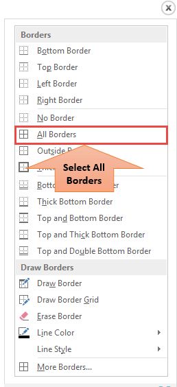
Select the option “All Borders”.
Your data should now look as follows

Tutorial Exercise 2
Using the knowledge gained above, try to change the font colour and try out other options available on the Home tab.