HLOOKUP Function
HLOOKUP stands for Horizontal Lookup and can be used to retrieve information from a table by searching a row for the matching data and outputting from the corresponding column. While VLOOKUP searches for the value in a column, HLOOKUP searches for the value in a row.
Formula
=HLOOKUP (value to look up, table area, row number)
How to use the HLOOKUP Function in Excel?
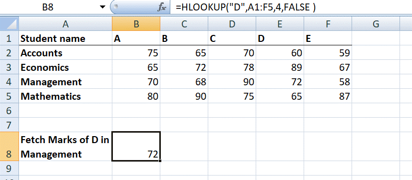
Let us consider the example below. The marks for four subjects for five students are as follows:

Now, if our objective is to fetch the marks of student D in Management, we can use HLOOKUP as follows:
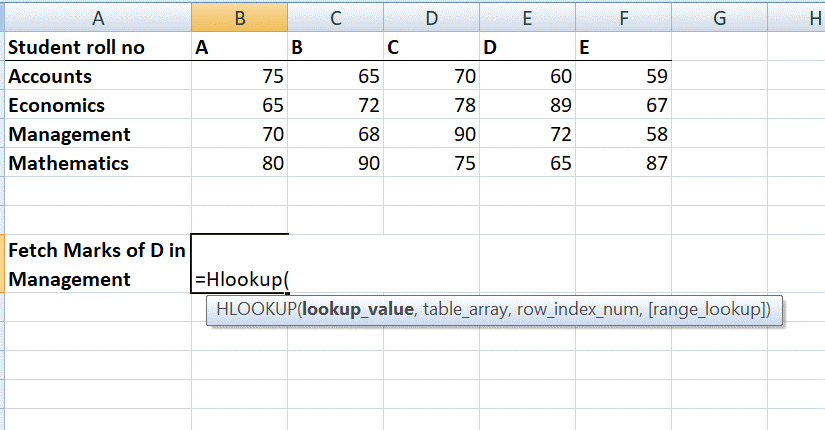
HLOOKUP function in Excel comes with the following arguments:
HLOOKUP(lookup_value, table_array, row_index_num, [range_lookup])
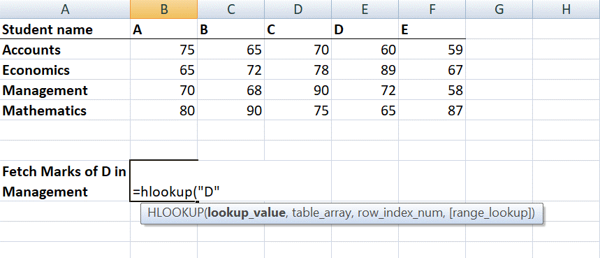
As you can see in the screenshot above, we need to give the lookup_value first. Here, it would be student D as we need to find his marks in Management. Now, remember that lookup_value can be a cell reference or a text string, or it can be a numerical value as well. In our example, it would be the student’s name as shown below:
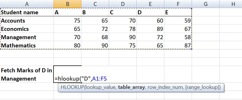
The next step would be to give the table array. A table array is nothing but rows of data in which the lookup value would be searched. A table array can be a regular range or a named range, or even an Excel table. Here we will give row A1:F5 as the reference.
Next, we would define ‘row_index_num,’ which is the row number in the table_array from where the value would be returned. In this case, it would be 4, as we are fetching the value from the fourth row of the given table.
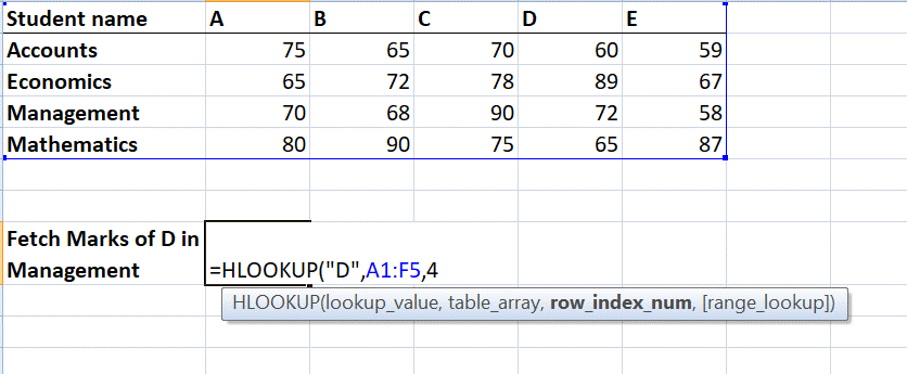
Suppose, if we require marks in Economics then we would put row_index_num as 3.
The next is range_lookup. It makes HLOOKUP search for an exact or approximate value. As we are looking out for an exact value, it would be False.
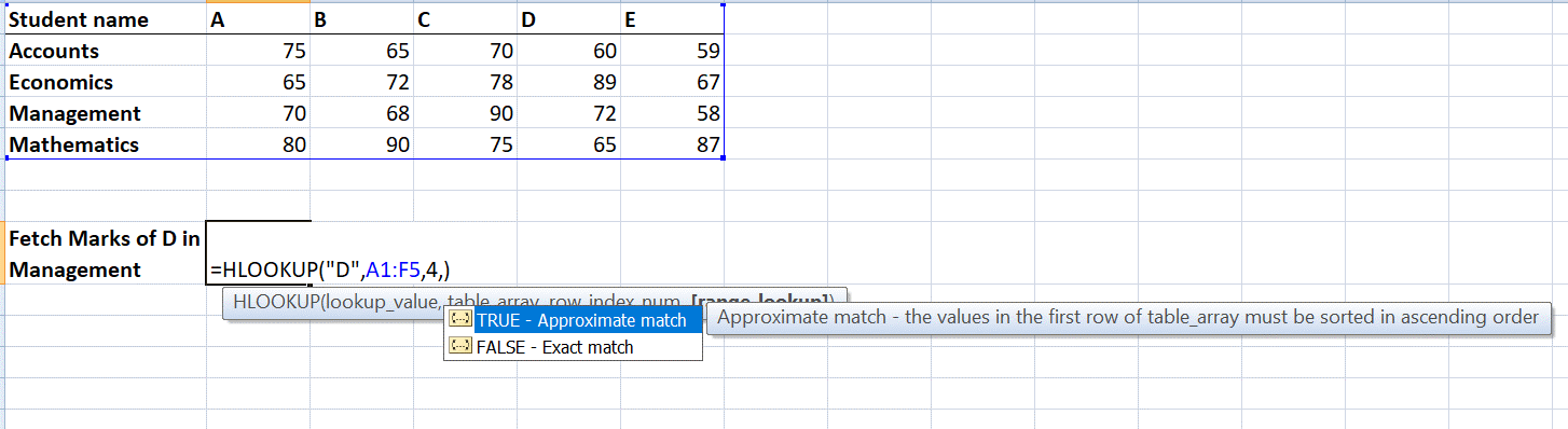
The result would be 72.