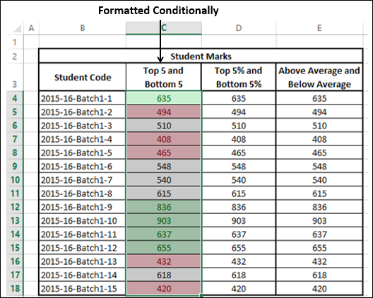
In Microsoft Excel, you can use Conditional Formatting for data visualization. You have to specify formatting for a cell range based on the contents of the cell range. The cells that meet the specified conditions would be formatted as you have defined.
You can specify any number of conditions for formatting by specifying Rules.
You can pick up the rules that match your conditions from
- Highlight cells rules
- Top / Bottom rules
You can also define your own rules. You can
- Add a rule
- Clear an existing rule
- Manage the defined rules
Further, you have several formatting options in Excel to choose the ones that are appropriate for your Data Visualization −
- Data Bars
- Color Scales
- Icon Sets
Conditional formatting has been promoted over the versions Excel 2007, Excel 2010, and Excel 2013.
Highlight Cells Rules
You can use the Highlight Cells rule to assign a format to cells whose contents meet any of the following criteria −
Numbers within a given numerical range −
- Greater Than
- Less Than
- Between
- Equal To
- Text that contains a given text string.
Date occurring within a given range of dates relative to the current date −
- Yesterday
- Today
- Tomorrow
- In the last 7 days
- Last week
- This week
- Next week
- Last month
- This Month
- Next month
- Values that are duplicate or unique.
Follow the steps to conditionally format cells –
- Select the range to be conditionally formatted.
- Click Conditional Formatting in the Styles group under the home tab.
- Click Highlight Cells Rules from the drop-down menu

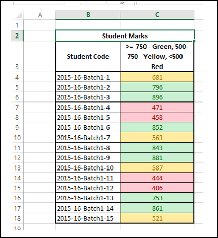
- Click Greater Than and specify >750. Choose a green color.
- Click Less Than and specify < 500. Choose a red color.
- Click Between and specify 500 and 750. Choose yellow color.

The data will be highlighted based on the given conditions and the corresponding formatting.
Top /bottom Rules
You can use Top / Bottom Rules to assign a format to cells whose contents meet any of the following criteria −
- Top 10 items − Cells that rank in the top N, where 1 <= N <= 1000.
- Top 10% − Cells that rank in the top n%, where 1 <= n <= 100.
- Bottom 10 items − Cells that rank in the bottom N, where 1 <= N <= 1000.
- Bottom 10% − Cells that rank in the bottom n%, where 1 <= n <= 100.
- Above average − Cells that are above average for the selected range.
- Below average − Cells that are below average for the selected range.
Follow the steps given below to assign the Top/Bottom rules.
- Select the range to be conditionally formatted.
- Click Conditional Formatting in the Styles group under the home tab.
- Click Top/Bottom Rules from the drop-down menu. Top/Bottom rules options appear.
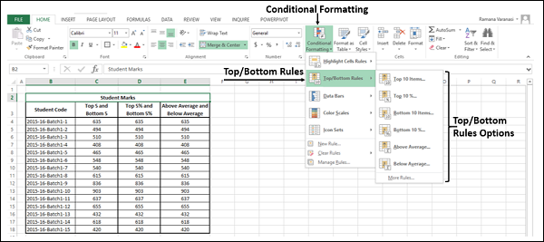
- Click Top Ten Items and specify 5. Choose green color.
- Click Bottom Ten Items and specify 5. Choose red color.
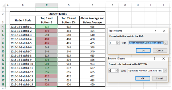
The data will be highlighted based on the given conditions and the corresponding formatting.

Repeat the first three steps given above.
Click Above Average. Choose green color.
Click Below Average. Choose red color.
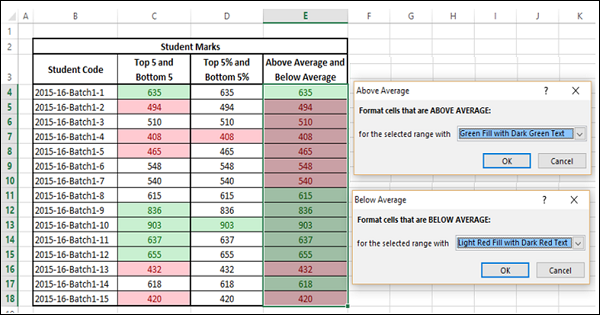
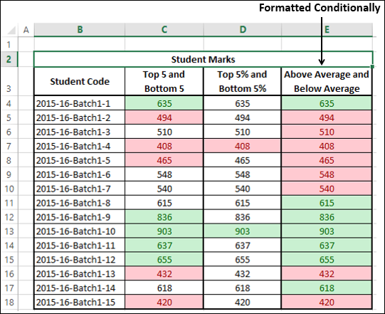
The data will be highlighted based on the given conditions and the corresponding formatting.