The Excel IFS function can run multiple tests and return a value corresponding to the first TRUE result. Use the IFS function to evaluate multiple conditions without multiple nested IF statements. IFS allows shorter, easier to read formulas.
USES
Test multiple conditions, return first true
Return value
Value corresponding with first TRUE result
Arguments
- test1 – First logical test.
- value1 – Result when test1 is TRUE.
- test2, value2 – [optional] Second test/value pair.
Syntax
=IFS (test1, value1, [test2, value2], …)
notes
The IFs function evaluates multiple expressions and returns a result that corresponds to the first TRUE result. You can use the IFS function when you want a self-contained formula to test multiple conditions at the same time without nesting multiple IF statements. Formulas based on IFS are shorter and easier to read and write.
Conditions are provided to the IFS function as test/value pairs, and IFS can handle up to 127 conditions. Each test represents a logical test that returns TRUE or FALSE, and the value that follows will be returned when the test returns TRUE. In the event that more than one condition returns TRUE, the value corresponding to the first TRUE result is returned. For this reason, it is important to consider the order in which conditions appear.
Structure
An IFS formula with 3 tests can be visualized like this:
=IFS (
test1,value1// pair 1
test2,value2// pair 2
test3, value3// pair 3
)
A value is returned by IFS only when the previous test returns TRUE, and the first test to return TRUE “wins”. For better readability, you can add line breaks to an IFS formula as shown above.
Note: the IFS function does not provide an argument for a default value. See Example #3 below for a workaround.
Example #1 – grades, lowest to highest
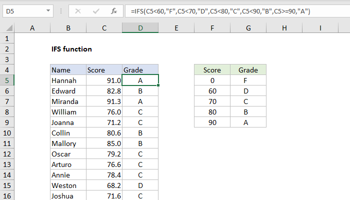
In the example shown below, the IFS function is used to assign a grade based on a score. The formula in E5, copied down, is:
=IFS (C5<60,"F",C5<70,"D",C5<80,"C",C5<90,"B", C5>=90,"A")
Notice the conditions are entered “in order” to test lower scores first. The grade associated with the first test to return TRUE is returned.
Example #2 – rating, highest to lowest
In a simple rating system, a score of 3 or greater is “Good”, a score between 2 and 3 is “Average”, and anything below 2 is “Poor”. To assign these values with IFS, three conditions are used:
=IFS (A1>=3,"Good",A1>=2,"Average",A1<2,"Poor")
Notice in this case conditions is arranged to test higher values first.
Example #3 default value
The IFS function does not have a built-in default value to use when all conditions are FALSE. However, to provide a default value, you can enter TRUE as a final test, followed by a value to use as a default.
In the example below, a status code of 100 is “OK”, a code of 200 is “Warning”, and a code of 300 is “Error”. Any other code value is invalid, so TRUE is provided as the final test, and “Invalid” is provided as a “default” value.
=IFS (A1=100,"OK",A1=200,"Warning",A1=300,"Error",TRUE,"Invalid")
When the value in A1 is 100, 200, or 300, IFS will return the messages shown above. When A1 contains any other value (including when A1 is empty) IFS will return “Invalid”. Without this final condition, IFS will return #N/A when a code is not recognized.