Filtering allows you to extract data that meets the defined criteria from a given Range or table. This is a quick way to display only the information that is needed by you.
You can Filter data in a Range, table, or PivotTable.
You can filter data by −
- Selected values
- Text filters if the column you selected contains text
- Date filters if the column you selected contains dates
- Number filters if the column you selected contains numbers
- Number filters if the column you selected contains numbers
- Font color if the column you selected contains font with color
- Cell icon if the column you selected contains cell icons
- Advanced filter
- Using slicers
In a table, the column headers are automatically tagged to filters, known as AutoFilters. AutoFilter is represented by the arrow next to the column header. Each AutoFilter has filter options based on the type of data you have in that column. For example, if the column contains numbers when you click on the arrow next to the column header, Number Filter Options appear.
When you click a Filter option or when you click on Custom Filter that appears at the end of the Filter options, the Custom AutoFilter dialog box appears, wherein you can customize your filtering options.
In the case of a Range, you can provide the column headers in the first row of the range and click on filter in the Editing group on the home tab. This will make the AutoFilter on for the Range. You can remove the filters that you have in your data. You can also reapply the filters when data changes occur.
Filter by Selected Values
You can choose what data is to be displayed by clicking the arrow next to a column header and selecting the Values in the column. Only those rows containing the selected values in the chosen column will be displayed.
Consider the following data –
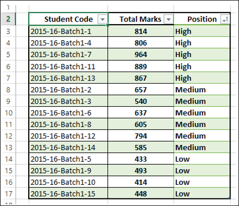
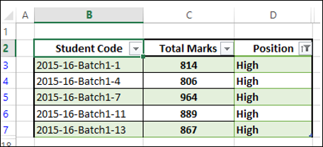
If you want to display the data only for Position = High, click the arrow next to Position. A drop-down box appears with all the values in the position column. By default, all the values will be selected.
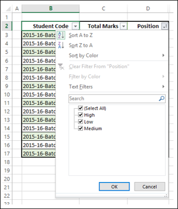
- Click Select All. All the boxes are cleared.
- Select High as shown in the following screen shot.
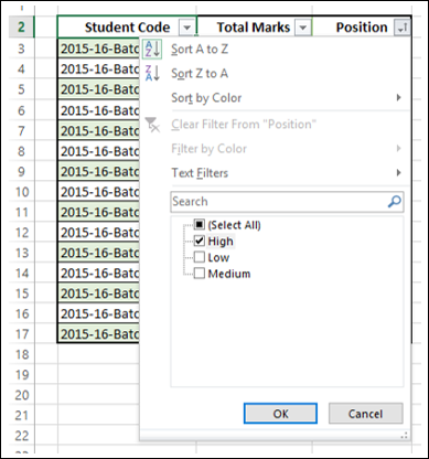
Click OK. Only those Rows, which have the value High as Position, will be displayed.
Filter by Text
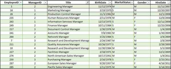
Consider the following data −
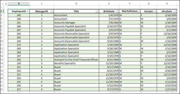
You can filter this data such that only those Rows wherein the Title is “Manager” will be displayed.
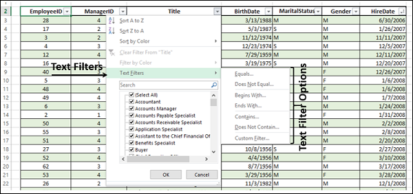
Click the arrow next to the column header Title. From the drop-down list, click Text Filters. Text filter options appear.
Select Contains from the available options. The Custom AutoFilter dialog box opens. Type Manager in the Box next to Contains.
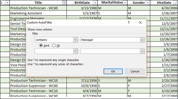
Click OK. Only the Rows where the Title contains the Manager will be displayed.