
Working with time series data can feel like trying to organize a library while the shelves are moving. In Python, however, we have specialized tools that turn “messy dates” into “predictable patterns.” This guide covers the journey from loading raw timestamps to generating meaningful forecasts.
What is Time Series Data?
Time series data is any data recorded at specific time intervals. Unlike standard tabular data, the order matters because each data point depends on what came before it.
Instead of treating dates as simple text strings, Python treats them as objects that understand the relationship between seconds, days, and years.
Why Python is Essential for Time Series
Using Python for time series helps you:
- Handle Missing Data: Automatically fill gaps in your timeline.
- Resample Easily: Convert daily data into monthly averages with one line of code.
- Visualize Trends: Identify seasonality and “noise” instantly.
- Scale Up: Process millions of timestamps faster than any spreadsheet.
Core Python Tools for Time Series
The “Big Three” libraries for this work are Pandas (for manipulation), Statsmodels (for analysis), and Prophet (for forecasting).
1. Converting Strings to Datetime
Raw data often arrives as text (e.g., “2024-01-01”). The first step is converting it into a datetime object using Pandas. Example: pd.to_datetime(df['date_column'])
- Useful for: Sorting data chronologically and extracting months or weekdays.
2. Resampling and Rolling Windows
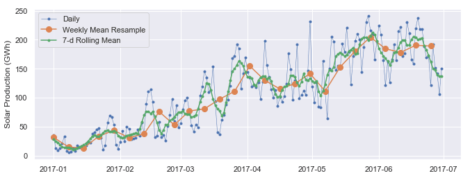
Resampling allows you to change the frequency of your data, while rolling windows help smooth out fluctuations. Example: df.resample('M').mean() — Aggregates data by month. df.rolling(window=7).mean() — Creates a 7-day moving average.
3. Decomposition: Breaking Down the Signal
Before forecasting, you must break a series into its component parts to understand what is actually happening.
- Trend: The long-term direction (up, down, or flat).
- Seasonality: Repeating patterns (like higher sales every December).
- Residuals: The random noise or “shocks” left over.
4. Stationary vs. Non-Stationary Data
Most statistical models require data to be stationary, meaning its mean and variance don’t change over time. If your data has a trend, you may need to use Differencing (subtracting the previous value from the current one) to stabilize it.
5. Forecasting with Prophet or ARIMA
Once the data is clean, you can predict the future. Example (Prophet): model.fit(df) future = model.make_future_dataframe(periods=365) This generates a forecast with confidence intervals, showing you the likely range of future values.
Combining Techniques for Better Insights
The real power comes from combining these steps into a single pipeline:
- Clean the data by filling missing dates (Interpolation).
- Filter for specific time ranges or holiday periods.
- Decompose to see the underlying trend vs. seasonal spikes.
- Forecast to plan for the next quarter with statistical confidence.
Advanced Feature Engineering
In time series, your best features are often derived from the time index itself:
- Lag Features: Using the value from “yesterday” to predict “today.”
- Window Statistics: Using the max or min value of the last 30 days.
- Date Attributes: Extracting whether a day is a weekend, holiday, or payday.
Common Challenges
If your analysis feels “off,” it’s often due to these common pitfalls:
- Timezone Mismatches: Mixing UTC with local time can shift your data incorrectly.
- Irregular Intervals: Missing data points can break forecasting models.
- Look-ahead Bias: Accidentally using future data to “predict” the past during model training.
Conclusion
Handling time series data in Python transforms raw, confusing timestamps into a crystal ball for your business or research. By moving away from manual date manipulation and embracing automated libraries, you can focus on the “why” behind the numbers rather than the “how” of the formatting.