
Introduction:
Data analysis is a crucial part of decision-making in various fields, from business and finance to research and marketing. However, working with large datasets can be overwhelming and time-consuming. This is where pivot tables in Excel and Google Sheets come to the rescue. Pivot tables are powerful tools that simplify data analysis, enabling you to quickly summarize and gain valuable insights from your data.
What is a pivot table?
A pivot table is a feature in spreadsheet software like Microsoft Excel and Google Sheets that allows you to reorganize and summarize your data easily. It enables you to transform rows of raw data into a more structured format, making it easier to extract meaningful information. Pivot tables are particularly useful when you have a lot of data and want to answer specific questions or spot trends.
Key Benefits of Pivot Tables:
- Simplifies Data Summarization: Pivot Tables make it effortless to summarize data by providing options to group, count, sum, average, or perform other calculations on your data.
- Flexible Data Exploration: You can quickly change the arrangement of your data to explore it from different angles, helping you uncover insights that might not be obvious in the raw data.
- Customizable Reporting: Pivot Tables allow you to create customized reports and charts, making it easy to communicate your findings to others.
- Time and Effort Savings: They eliminate the need for manually sorting and calculating data, saving you a significant amount of time and effort.
How to Create a Pivot Table:
- Prepare Your Data: Ensure your data is organized in a tabular format with column headers. Remove any empty rows or columns. We will make use of this sample data
Sample Data
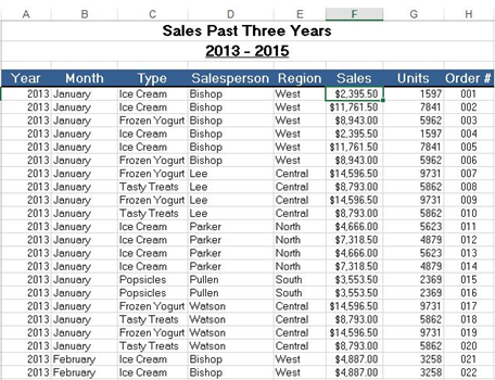
The sample data that we are going to use contains 448 records with 8 fields of information on the sale of products across different regions between 2013-2015. This data is perfect to understand the pivot table.
2.Select your data: Highlight the range of data you want to analyze.
- Insert a Pivot Table: In Excel, go to the “Insert” tab and click on “Pivot Table.” In Google Sheets, go to “Data” and select “Pivot table.”

- A dialog box will appear. Excel will auto-select your dataset. It will also create a new worksheet for your pivot table.
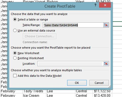
Click Ok. Then, it will create a pivot table worksheet.
4.Configure your pivot table: Drag and drop the fields (columns) into the appropriate areas of the pivot table builder: Rows: The categories by which you want to group your data. Additional data categorization if needed Values The data you want to summarize (e.g., salesperson, Sales).Filters: Filters to narrow down the data you want to analyze.
- Drag Field
To get the total sales of each salesperson, drag the following fields to the following areas.
- Salesperson field to Rows area.
- Sales field to Values area.
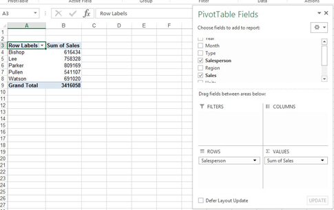
- Value Field Settings
By default, Excel gives the summation of the values that are put into the Values section. You can change that from the Value Field Settings.
- Click on the Sum of Sales in the Values field.
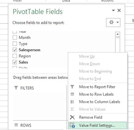
- Choose the type of calculation you want to use

- Click OK
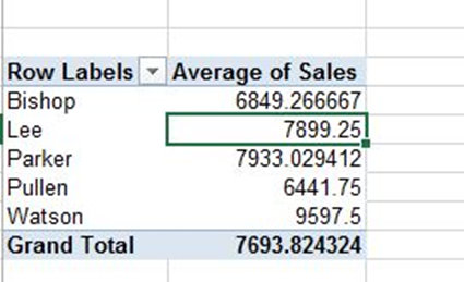
- Sorting By Value
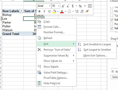
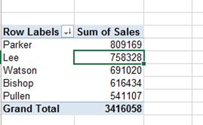
- Right-click any Sales value and choose Sort > Sort Largest to Smallest.
Result:
Conclusion
In this article, you’ve learned the basics of pivot table creation in Excel. You can see how simple it is to get started creating one and visualizing your data in many different ways.
One of the best way to Boost your analytic career is to get the right place to acquire your skill. At Megatek ICT Academy, we take you from novice to pro.
Check out www.ictacademy.com.ng for more info Or call 08033146625