
For many Excel users, VLOOKUP is the go-to function for searching data. While it is useful, it has several limitations that can make your spreadsheets inefficient and difficult to scale.
This is where INDEX and MATCH come in.
INDEX and MATCH provide a more flexible, powerful, and reliable way to perform lookups in Excel. Professionals and data analysts prefer this combination because it overcomes many of the weaknesses of VLOOKUP.
In this article, you’ll learn how INDEX and MATCH work, why they are better, and how to use them effectively.
Why VLOOKUP Falls Short
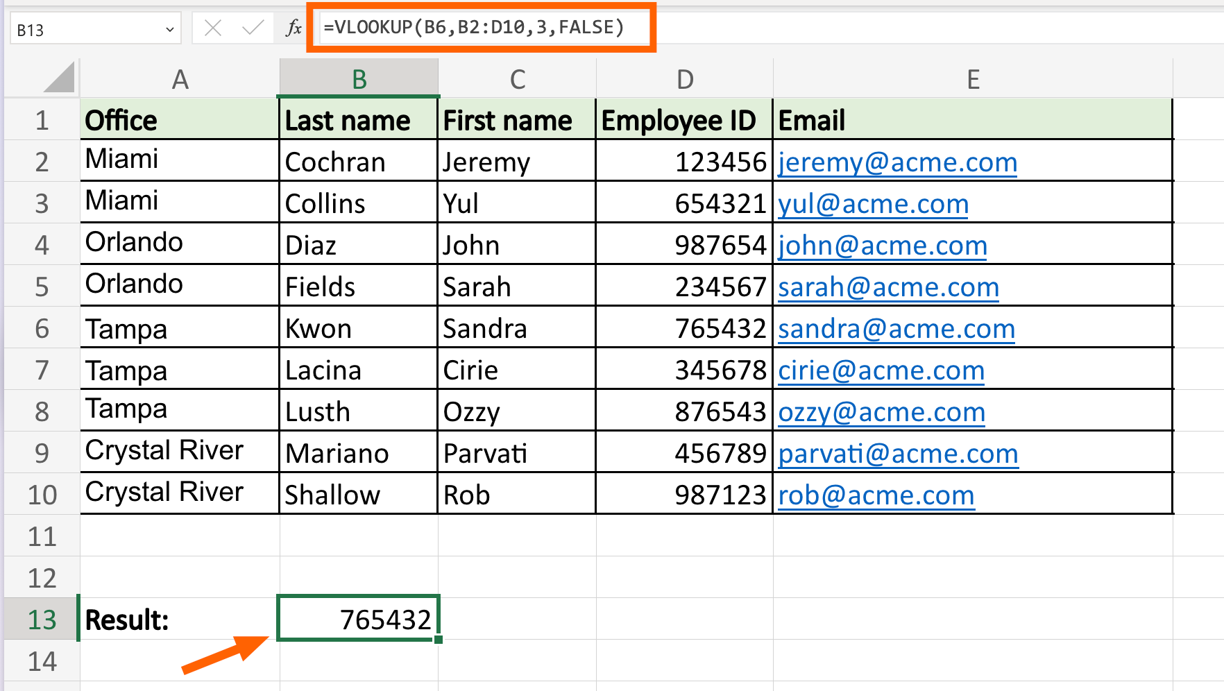
Before diving into INDEX and MATCH, it is important to understand the limitations of VLOOKUP.
Some common issues include:
- It only searches from left to right
- It breaks when columns are rearranged
- It requires column index numbers
- It is less efficient with large datasets
For example, if your lookup value is not in the first column, VLOOKUP cannot retrieve the data without restructuring your table.
What is the INDEX Function?
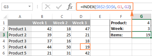
The INDEX function returns a value from a specific position in a table or range.
Syntax:
=INDEX(array, row_num, [column_num])
What It Does:
- Retrieves a value based on its position
- Works with both rows and columns
Example:
=INDEX(A2:C10, 3, 2)
This returns the value in the 3rd row and 2nd column of the range.
What is the MATCH Function?
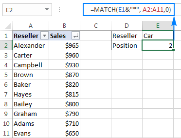
The MATCH function searches for a value and returns its position.
Syntax:
=MATCH(lookup_value, lookup_array, [match_type])
What It Does:
- Finds the position of a value in a range
- Works horizontally or vertically
Example:
=MATCH("John", A2:A10, 0)
This returns the position of “John” in the range.
Combining INDEX and MATCH
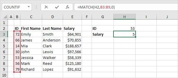
The real power comes when you combine both functions.
Formula:
=INDEX(B2:B10, MATCH("John", A2:A10, 0))
What This Does:
- MATCH finds the position of “John”
- INDEX returns the corresponding value from another column
This combination replaces VLOOKUP and offers greater flexibility.
Advantages of INDEX and MATCH Over VLOOKUP
INDEX and MATCH provide several advantages:
- Works in any direction (left or right)
- Does not break when columns are moved
- More efficient with large datasets
- More flexible and dynamic
These advantages make it the preferred choice for advanced Excel users.
Two-Way Lookup with INDEX and MATCH
You can also perform two-dimensional lookups.
Example:
=INDEX(B2:E10, MATCH("Product A", A2:A10, 0), MATCH("March", B1:E1, 0))
What It Does:
- Finds the row using MATCH
- Finds the column using another MATCH
- Returns the intersecting value
This is something VLOOKUP cannot easily handle.

Common Mistakes to Avoid
When using INDEX and MATCH, avoid these mistakes:
- Using incorrect ranges
- Forgetting to use 0 for exact match
- Mixing up row and column references
- Not locking ranges when copying formulas
Always double-check your references for accuracy.
Best Practices
To use INDEX and MATCH effectively:
- Use named ranges for clarity
- Keep lookup columns clean and consistent
- Always use exact match unless necessary
- Test formulas before applying across datasets
These practices ensure reliable results.
Conclusion
While VLOOKUP is popular, it has limitations that can restrict your ability to work efficiently with data. INDEX and MATCH provide a more powerful and flexible solution for performing lookups in Excel.
By mastering INDEX and MATCH, you can build more dynamic spreadsheets, handle complex datasets, and work like a professional data analyst.
Once you start using INDEX and MATCH, you may never go back to VLOOKUP.