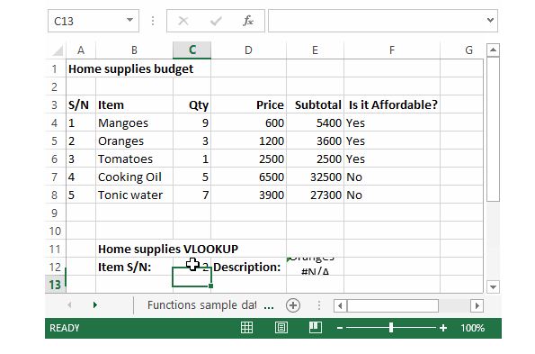
The VLOOKUP function is used to perform a vertical look up in the left most column and return a value in the same row from a column that you specify. Let’s explain this in a layman’s language. The home supplies budget has a serial number column that uniquely identifies each item in the budget. Suppose you have the item serial number, and you would like to know the item description, you can use the VLOOKUP function. Here is how the VLOOKUP function would work.

=VLOOKUP (C12, A4:B8, 2, FALSE)
HERE,
- “=VLOOKUP” calls the vertical lookup function
- “C12” specifies the value to be looked up in the left most column
- “A4:B8” specifies the table array with the data
- “2” specifies the column number with the row value to be returned by the VLOOKUP function
- “FALSE,” tells the VLOOKUP function that we are looking for an exact match of the supplied look up value
The image below shows this in action