Welcome to another tutorial from Megatek ICT Academy, today we are going to be talking about conditional formatting for numbers, in another tutorial we talked about conditional formatting for text.
In this tutorial we are going to be learning how to differentiate number from another using colors, for example the average mark needed for a student to pass is 50; so we are going to format numbers from 50-100(Pass) so it can be differentiated from 0-49 (Fail).
Let’s get on with it then.
- Firstly you need to have an open excel filled with result of students
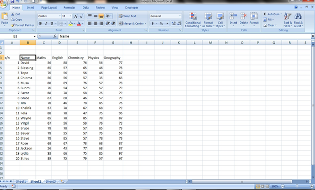
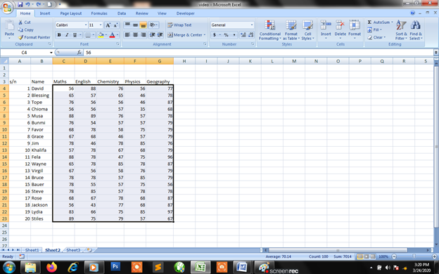
- Highlight all the cell you want to format or you can do it individually works the same way. We are going to be taking all the cells with numbers at once.
N.B
Highlight only the cell you want to format. DO NOT Highlight the headers or in our case the subject with it

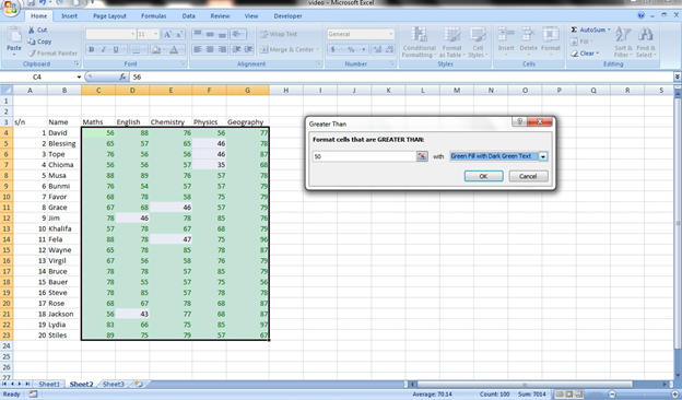
- As we have highlighted the cells we click on conditional formatting on the Home tab under styles, select the Highlight cell rules, click the greater than
- It gives a pop up dialog box that asks you to format cell greater than in our case 50 and we are giving it a green fill with dark green text
- With the cells still highlighted do the same for less than 50

- If you followed the above steps you are bound to have the below result
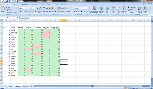
From the above result you can see that numbers from 50-100 are formatted green to denote that they passed while the numbers below 50 (0-49) are formatted red to show they Failed.

interesting
understandable